Using Genetic Programming to Play Mancala

      This paper will explain what genetic programming is, what mancala is, how I used genetic programming to evolve mancala-playing programs, and the results I got from doing so.

What is Genetic Programming?

      Genetic programming is an automatic programming technique - that is, a method for generating computer programs other than having a human write them - inspired by and roughly modeled on biological evolution. John R. Koza of Stanford University is generally considered the inventor of genetic programming, although there were a number of related techniques that preceded his discovery, most notably genetic algorithms (which were invented by John Holland at the University of Michigan in 1975). An outline of the genetic programming process follows:

1. Generate the initial population
2. Evaluate the fitness of the population
3. Generate the next generation of the population
   1. Select a member of the previous generation, weighting the choice based on the fitness of the solutions
   2. If appropriate, perform crossover
   3. If appropriate, perform mutation
   4. Add that solution to the next generation
   5. Repeat a-d until the next generation is full
4. Repeat 2-3 until finished

      This outline is essentially the same process that is used in genetic algorithms. The difference is that genetic algorithms are generally performed on bit strings, whereas genetic programming works on programs or virtual programs. The process will be described in more detail during the discussion of how this project was implemented.

The Game of Mancala

      The project that was decided on was to use genetic programming to evolve programs to play the game mancala. Mancala (also called Owari) is a two-player ancient African board game with many different variations. A mancala board is a board with 14 bowls carved into it.

Figure 1. A mancala board.

      As shown in Figure 1, the mancala board is initially set up with four stones in each of the small bowls. The larger bowls on either end of the board are called the mancalas. The rules for mancala as they were used in this project are as follows:

1. A move consists of picking up all of the stones in one of the bowls on the player's side of the board (excluding the mancalas,) and then going counter-clockwise around the board, placing one stone in each bowl until all the stones have been placed. When placing stones, a player places a stone in the mancala on his right, but - if he gets to it - he skips the mancala on his left. (The players sit on opposite sides of the board.) See Figure 2.
2. Whenever the last stone in a move is placed in the mancala, the player gets to immediately take another move.
3. If the last stone in a move is placed in an empty bowl on the moving player's side of the board, that stone, and any stones in the bowl directly across from the bowl the last stone was placed in, are all placed in the moving player's mancala (i.e., the one on the player's right.)
4. If all six bowls on one side of the board are ever empty, the player who still has stones on his side of the board may pick up all of the stones in his six cups and place them in his mancala. The game is then over.
5. The players take turns making moves until all of the stones are in the mancalas. The winner is the player with the most stones in his mancala.

Figure 2. The resolution of an example first move of the game.

Implementing Genetic Programming to Play Mancala

      Figure 3 is a list of all the major parameters used in this project. (It's called a Koza Tableau after it's creator). Note that this project was actually run twice, and the two runs were not identical. In the second run, the method for determining fitness was altered (more on this later).

      One of the most common ways of representing programs in genetic programming is as trees. For this project, tree objects were written in C++ to represent the programs. The functions used were addition, subtraction (both of which have two child nodes), value_at (which returns the number of stones at a given location, and has one child node), and an if_<_do_else_ function (which has four child nodes, and returns the value returned by the third child node if the first child node is less than the second child node; otherwise it returns the fourth child node). All of the terminal nodes were integers from 0 to 13.

Figure 4. An example program.

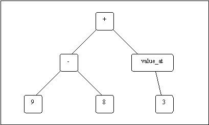
      Figure 4 shows a simple example of a program that might be generated during a run of the program. It returns the value (9-8) + value_at(3), or one plus however many stones are at the third bowl on the board. Whenever it's time for the generated program to take a turn in a game of mancala this value will be calculated and interpreted as the cup that it wants to move.

      To create the initial population, 512 programs such as the one depicted in Figure 4 were randomly created. Initial programs didn't exceed a depth of 16.

      To evaluate the fitness of each program, two games of mancala were run between it and the depth-first search algorithm - one in which the depth-first search went first, and one in which it went second. In the first run, the program was then assigned a fitness value equal to the sum of its scores in each game. In the second run, it was assigned a fitness value equal to that sum times 100 minus the number of nodes in the program (if this would result in a non-positive value, the fitness was set to 1).

      After all of the fitness values were calculated, the next generation of the population was created. First of all, the program with the highest fitness value is copied into the next generation. This is called elitism, and ensures that at the very least, each generation has a solution as fit as the previous generation, if not better. We're sure never to lose the progress we've made that way.

      To fill out the rest of the members of the population for the next generation, a member of the previous generation is selected at random. In this selection, each member has a chance to be selected proportional to its fitness. The probability that a given program will be selected is equal to its fitness value divided by the sum of all fitness values in the population. The selected program then has a 90% chance of having crossover performed on it, and a 0.5% chance of being mutated.

      Crossover and mutation are how our population is diversified. They are the motor that propels us through the search space of all possible programs. If crossover occurs, another member of the previous generation is selected as before. A subtree is selected at random from this other program and is added to the first program in place of one of its subtrees. If mutation occurs, a node of the program is selected at random. All of its child nodes are deleted and new children are created for it at random.

      The program is now added to the next generation of the population. This process of selecting programs from the previous generation, and then using crossover and mutation as necessary, is completed until the new generation is filled out. This new generation then in turn has its fitness evaluated, and the process continues.

      Both runs of the project resulted in programs that could defeat the eight-level depth-first search algorithm whether it went first or not. The best fit members of both of their final generations are presented in Figure 5.

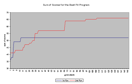
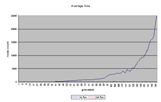
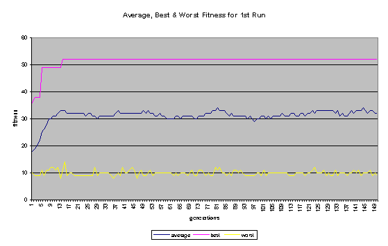
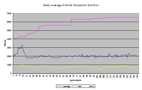
      On the whole, the second run was more successful. In the first run, the programs quickly became bloated (as shown in Figure 7), and no further improvement was evolved after the 14th generation. In the second run - where a penalty for large program size was built into the fitness function - the average program size remained comparatively low (never getting much higher than 100 nodes). The second run continued to improve until past generation 100 and ended up evolving a program that did substantially better than the best program to come out of the first run. A comparison in Score1 + Score1 for the best program of each generation for the two runs is shown in Figure 6. Some general fitness information about both runs can be found in Figures 8 and 9.

Figure 6.

Figure 7.

Figure 8.

Figure 9.

      The best solution that was found (in the second run) just barely squeaked by the DFS algorithm when it went second (25-23) but it won by a wide margin when it was allowed to go first (41-7). Not only that, but it's much more efficient that an eight-level depth-first search. The DFS has to step through on the order of 68 (1,679,616) possible moves. The final program for the second run, on the other hand, only has a total of 80 nodes.

      It's important to note, however, that this program is not a generally good mancala player. It only does this well against one specific opponent strategy that it has evolved to defeat. To prove this point, the DFS was run against 1,000 randomly created programs. The final program from each run were both then run against the same 1,000 programs. The results are quite telling (and can be seen in Figure 10). The DFS algorithm tended to win against the random programs with little problem. The evolved programs had trouble even tying. The DFS may be a generally good algorithm for playing mancala, but evolving a solution to beat it doesn't necessarily produce a solution that is a generally good algorithm. The evolved program may seize onto seemingly accidental facts about the state of the board when it plays against the DFS to determine which moves to make. When it plays an opponent that doesn't make the exact same moves, it doesn't work. To evolve a program that does well against a wide variety of opponents, it may be necessary for the fitness function to include playing against a number of different opponents.

      Another thing to note is that the best fit program from the second run doesn't use the if_<_do_else_ operator at all. In any future runs, it may be wise to remove this function entirely. The more functions there are, the more possible solutions there are to search through. Adding unnecessary functions may only serve to slow down the process of finding optimal solutions.